Functionals
A functional is a mapping of a normed linear space of functions (a Banach space) \(M\) of continuous functions \(f\) to the value of the function at a point \[\begin{equation} F : M \mapsto \mathbb{R} \text{ or } \mathbb{C} \thinspace . \end{equation}\] In a simple manner of speaking, a functional is a function of which the variable is a function. In quantum chemistry, functionals play an important, but sometimes hidden, role. For instance: the expectation value of the Hamiltonian \(\require{physics} \expval{\hat{H}}{\Psi}\) is a functional. Given \(\Psi\), one gets a number from this prescription. Similarly, \(\require{physics} \braket{\Psi}{\Psi}\) is a functional of \(\Psi\) such that the variational method is the search for the minimum of a functional (Parr and Yang 1989).
Functional derivative
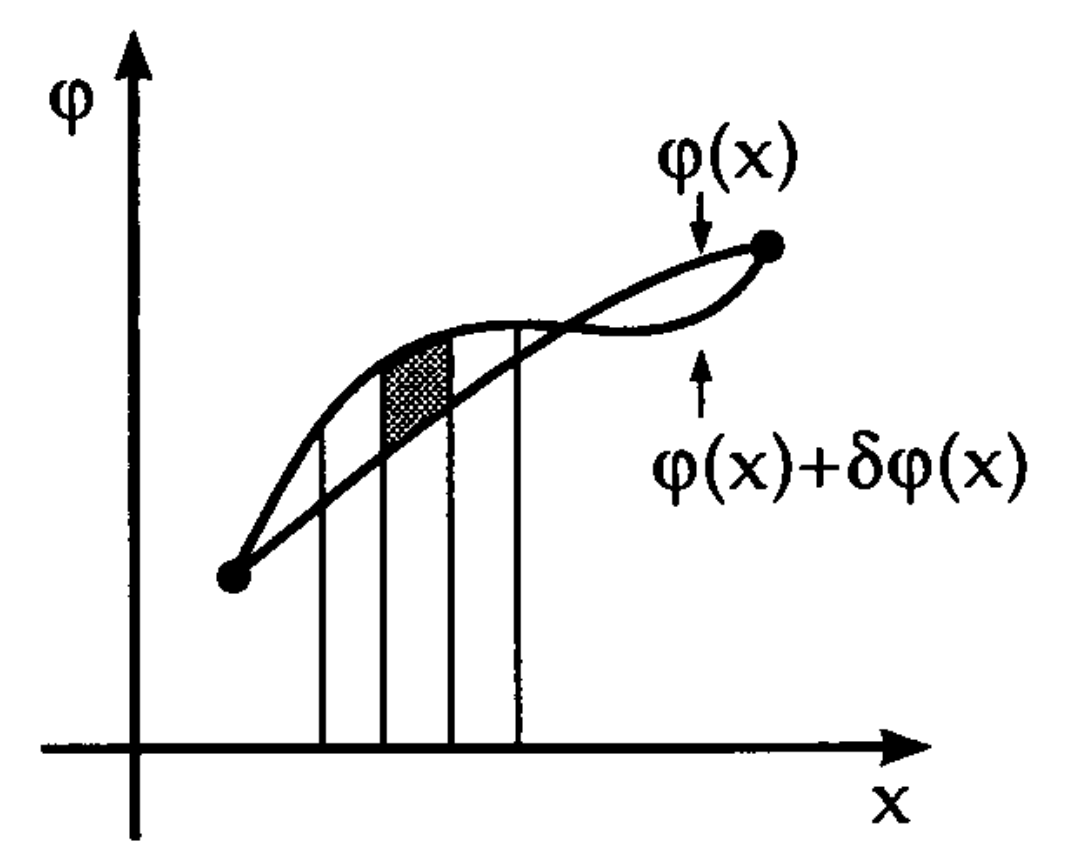
To find the function \(f(x)\) that finds the extremum of a given functional \(F[f]\), we need to define and evaluate its functional derivative (Parr and Yang 1989; Engel and Dreizler 2011). A variation of any function \(f\) by an infinitesimal amount can be represented in the form \[\begin{equation} \require{physics} \var{ f (x) } = \epsilon \eta(x) \thinspace , \end{equation}\] where the quantity \(\epsilon\) is an infinitesimal number and \(\eta\) is an arbitrary function. If we vary \(f\) by amount \(\var{F}\), the variation of the functional \(F\) becomes \[\begin{equation} \var{F} := F[ f + \var{f} ] - F[f] \thinspace . \end{equation}\] The technique used to evaluate \(\var{F}\) is a Taylor expansion of the functional \[\begin{equation} F[ f + \var{f} ] = F[ f + \epsilon \eta ] \end{equation}\] in powers of \(\var{f}\) or \(\epsilon\) respectively. The expansion of \(F[ f + \epsilon \eta ]\) is an standard Taylor expansion of the form \[\begin{align} F[ f + \epsilon \eta ] &= F[f] + \pdv{ F[ f + \epsilon \eta ] }{\epsilon} \Bigg|_{\epsilon=0} \epsilon + \frac{1}{2} \pdv[2]{ F[ f + \epsilon \eta ] }{\epsilon} \Bigg|_{\epsilon=0} \epsilon^2 + \dots \\ &= \sum_{n=0}^N \frac{1}{n!} \pdv[n]{ F[ f + \epsilon \eta ] }{\epsilon} \Bigg|_{\epsilon=0} \epsilon^n + \mathcal{O}( \epsilon^{n+1} ) \thinspace , \end{align}\] where the first-order expansion term is related to the functional derivative \(\fdv*{F[f]}{f(x_1)}\) as \[\begin{equation} \pdv{ F[ f + \epsilon \eta ] }{\epsilon} \Bigg|_{\epsilon=0} =: \int \dd{x_1} \fdv{F}{f(x_1)} \eta(x_1) \thinspace . \end{equation}\] This definition can be interpreted as: the total change in \(F[f]\) upon variation of the function \(f(x_1)\) is a superposition of the local changes summed over the whole range of \(x_1\) values (see figure above) (Greiner and Reinhardt 1996). The above definition can be thought of as an extension of the first total differential of a function \[\begin{equation} \dd{f} = \sum^N_n \pdv{f}{x_n} \dd{x_n} \end{equation}\] to the case of an inifite set of variables \(x_n\). The definition of the \(n\)-th order expansion term is \[\begin{equation} \pdv[n]{ F[ f + \epsilon \eta ] }{\epsilon} \Bigg|_{\epsilon=0} \epsilon =: \int \dd{x_1}, \dd{x_2} \dots \dd{x_n} \frac{ \delta^n F[f] }{ \delta f(x_1) \delta f(x_2) \dots \delta f(x_n) } \eta(x_1) \eta(x_2) \dots \eta(x_n) \thinspace . \end{equation}\] Rewriting the Taylor expansion in terms of its functional derivatives gives \[\begin{equation} F[ f + \epsilon \eta ] = \sum_{n=0}^N \frac{1}{n!} \int \dd{x_1}, \dd{x_2} \dots \dd{x_n} \frac{ \delta^n F[f] }{ \delta f(x_1) \delta f(x_2) \dots \delta f(x_n) } \eta(x_1) \eta(x_2) \dots \eta(x_n) + \mathcal{O}(\epsilon^{n+1}) \thinspace , \end{equation}\] with \(N\) being either finite or infinite. The differential of the functional \(F\) now becomes \[\begin{equation} \var{F} = \sum_{n=1}^N \frac{1}{n!} \int \dd{x_1}, \dd{x_2} \dots \dd{x_n} \frac{ \delta^n F[f] }{ \delta f(x_1) \delta f(x_2) \dots \delta f(x_n) } \eta(x_1) \eta(x_2) \dots \eta(x_n) + \mathcal{O}(\epsilon^{n+1}) \thinspace . \end{equation}\] If we only take the first order of the expansion into account, the differential is approximated to \[\begin{equation} \var{F} = \int \dd{x} \fdv{F}{f(x)} \eta(x) \thinspace , \end{equation}\] where we have replaced the integration over \(x_1\) with \(x\) for the sake of an uncluttered notation.
Calculational properties
For the practical evaluation of functional derivatives relevant in physics, a variation in terms of the \(\delta\)-function is used instead of \(\eta(x)\) \[\begin{equation} \eta(x) = \delta(x-x_1) \thinspace , \end{equation}\] which gives \[\begin{equation} \var{ F[f] } = F[f + \epsilon \var(x - x_1)] - F[f] = \int \dd{x} \fdv{F}{f(x)} \epsilon \delta(x - x_1) = \epsilon \fdv{F}{f(x_1)} \end{equation}\] or in the limit of vanishing \(\epsilon\) (and thus vanishing change in \(f(x)\)) \[\begin{equation} \fdv{F}{f(x_1)} = \lim_{\epsilon \to 0} \frac{ F[f + \epsilon \var(x - x_1)] - F[f] }{\epsilon} \thinspace . \end{equation}\] This relation is equivalent to the definition of \(\var{F}\), but is better suited for the practical evaluation of functional derivatives.
Since the functional derivatives constitute an extension of the concept of the ordinary derivative, most of the rules for ordinary derivatives can be incorporated for functional derivatives:
Linearity: \[\begin{equation} \fdv{ (C_1 F + C_2 G)[f] }{f(x)} = C_1 \fdv{ F[f] }{ f(x) } + C_2 \fdv{ G[f] }{ f(x) } \thinspace , \end{equation}\] where \(C_1\) and \(C_2\) are constants.
Product rule: \[\begin{equation} \fdv{ (F_1 F_2)[f] }{ f(x) } = \fdv{F_1[f]}{f(x)} F_2[f] + F_1[f] \fdv{F_2[f]}{f(x)} \thinspace , \end{equation}\]
Chain rule: \[\begin{equation} \fdv{}{f(x_1)} F[ G[f] ] = \int \dd{x} \fdv{F[G]}{G(y)} \fdv{G[f](y)}{f(x)} \thinspace . \end{equation}\]