Functions

Naturally, if we have two different sets, we would like to be able to define relations between their elements. This is exactly what a function does. A function (or map, mapping, these are all synonyms) is a relation between two sets \(X\) and \(Y\): \[\begin{equation} \label{eq:def_function} \require{physics} f: X \rightarrow Y: x \mapsto y = f(x) , \end{equation}\] subject to the important condition that every input \(x \in X\) is related to exactly one output \(y \in Y\). We would read the definition in equation \(\eqref{eq:def_function}\) as follows: \(f\) is a function from the set \(X\) to the set \(Y\), in which every \(x \in X\) is related to a \(y \in Y\), which we call \(f(x)\).

We give special names to the sets \(X\) and \(Y\), depending on which role they play in the function. The set \(X\) is called the domain of the function: it is the set of all inputs for the function. The set \(Y\) is then called the function’s codomain: it is the set of values that occur as output values for the function. We can then define another set, \(Z\), which is called the image of the function: it is the set of values for the outputs. A visual clarification of the terms can be found in Figure \(\ref{fig:functions}\).

Figure: functions

An example of a function could be: \[\begin{equation} f: \mathbb{R} \rightarrow \mathbb{R}: x \mapsto f(x) = x^2 + 2 \end{equation}\] Its domain is \(\mathbb{R}\), and its codomain is also \(\mathbb{R}\). Here, we can also see the difference between the codomain and the image. The codomain of this function is defined to be \(\mathbb{R}\), but its image \([2, +\infty[\). Another example is shown in Figure \(\ref{fig:function_color}\).

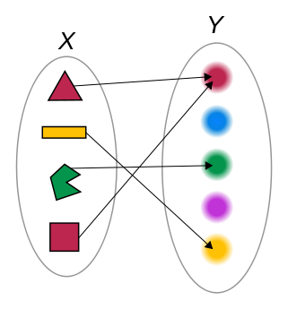
A function that maps its elements to their colors.

The reason why this is a function is because every input element of the set \(X\), being shapes in a certain color, is related to its color, represented as elements of the set \(Y\). In this case, \(Y\), the codomain is the set of colors depicted as elements of \(Y\), and the range is the set of colors red, green and yellow.

We have seen some examples of functions already, but what are some examples relations that are not functions? There are actually two requirements to the definition of a function:

With these two criteria in mind, it is possible to come up with many examples of relations between two sets that are not functions, for example those shown in Figure \(\ref{fig:non_functions}\).

Examples of non-functions

The identity function on a set \(S\) is the function: \[\begin{equation} \text{id}_S: S \rightarrow S: \text{id}_S(s) = s \thinspace . \end{equation}\]

An operation can hardly be distinguished from the definition of a function that was already given. It is a function \[\begin{equation} \omega: Y_1 \times \cdots \times Y_N \rightarrow X \thinspace , \end{equation}\] which takes as an input one element of every of its input sets \(Y_i\) and relates that combination to the output set \(X\). For me, this definition is exactly equal to the definition that was given previously. However, it seems that the term operation is often used to talk about associativity, commutativity, etc.

We know many operations, for example number addition, which takes two numbers as input and relates that combination to a number. Number multiplication is another example of a binary operation: we take two numbers, whose product is a number. If we take, for example, set of \(n \times n\) matrices, then matrix multiplication is an example of a binary operation. Furthermore, we don’t have to take inputs from the same sets! We can define scalar multiplication as an operation that relates a number and a vector to a vector.

By now, we have seen some examples of functions. In order to classify functions, we will introduce the terms surjection, injection, and bijection. For a visual overview of the terms, see Figure \(\ref{fig:sur_in_bi}\).

A function is called surjective (or: onto), if every element of its codomain is mapped to. means `above’, which relates to the fact that the function’s codomain is completely covered. Its definition can be written as follows: a function \(f\) is said to be surjective if \[\begin{equation} f: X \rightarrow Y: \forall y \in Y: \exists x \in X: f(x) = y \thinspace . \end{equation}\]

A function is called injective (or: one-to-one) if no element of its codomain is mapped to twice. Mathematically, we would write: \(f\) is an injective function if \[\begin{equation} f: X \rightarrow Y: \forall a, b \in X: f(a) = f(b) \Rightarrow a = b \thinspace . \end{equation}\]

A function is called bijective (or: one-to-one and onto, a one-to-one correspondence), if it is both injective and surjective: every element of the codomain is mapped to by exactly one element of the domain.

A visual scheme of the terms surjective, injective and bijective.

Given Figure \(\ref{fig:sur_in_bi}\), we can already see examples of surjective and injective functions. In Figure \(\ref{fig:function_color}\), we can see an example of a function that is not surjective (not every color is mapped to), nor injective (the color red is mapped to twice).